
Binary Decision Diagrams (BDDs) are a powerful data structure used to represent and manipulate Boolean functions efficiently. First introduced in their modern reduced form by Randal Bryant in 1986, they became one of the most important data structures in computer science — powering formal verification, digital circuit design, model checking, and AI reasoning. Their key strength is representing enormous Boolean functions compactly, and performing operations directly on that compact form without ever expanding it.
This guide explains what a BDD is, how the reduction rules turn a decision tree into a compact diagram, the difference between OBDDs and ROBDDs, how BDDs compare to binary decision trees and binary search trees, a working C example, real-world applications, and the main libraries used in practice.
The C example in this guide compiles cleanly under the C11 standard (GCC, -Wall -Wextra) and was tested to produce the output shown.
What Is a Binary Decision Diagram?
A Binary Decision Diagram (BDD) is a rooted directed acyclic graph (DAG) that represents a Boolean function. It has two kinds of nodes:
- Decision nodes, each labeled with a Boolean variable, with two outgoing edges: a low edge (taken when the variable is 0) and a high edge (taken when the variable is 1).
- Terminal nodes (leaves), each labeled either 0 (False) or 1 (True), representing the final value of the function.
To evaluate the function for a given assignment of variables, you start at the root and follow the low or high edge at each decision node according to that variable’s value, until you reach a terminal. The terminal’s value is the function’s result.
NIST defines a Binary Decision Diagram as “a binary lattice data structure that succinctly represents a truth table by collapsing redundant nodes and eliminating unnecessary nodes.”
Because operations can be performed directly on this compressed graph — conjunction (AND), disjunction (OR), and negation (NOT) — without ever decompressing it back to a truth table, BDDs can handle Boolean functions with hundreds of variables that would be impossible to store as explicit truth tables.
Key Features of BDDs
- Compact representation. BDDs represent large Boolean functions compactly by sharing identical subgraphs instead of duplicating them.
- Canonical form. A Reduced Ordered BDD (ROBDD) is canonical — for a fixed variable order, every Boolean function has exactly one ROBDD. This makes checking whether two functions are equal as simple as checking whether their ROBDDs are identical.
- Efficient operations. BDDs support efficient Boolean operations (AND, OR, NOT) and quantification, all performed directly on the graph.
From Truth Table to Decision Tree
Every Boolean function can be written as a truth table listing its output for each combination of inputs. It can also be drawn as a binary decision tree: starting from the first variable, each level branches on one variable (0 to the left, 1 to the right) until reaching a leaf that gives the output.
For example, consider a function f(x1, x2, x3). Following an assignment like x1=0, x2=1, x3=1 means starting at x1, taking the low (dashed) edge because x1=0, then two high (solid) edges because x2=1 and x3=1, arriving at a terminal that gives the function’s value for that input.
The problem with a full decision tree is that it grows exponentially — a function of n variables has a tree with 2ⁿ leaves. That’s where reduction comes in.
The Two Reduction Rules
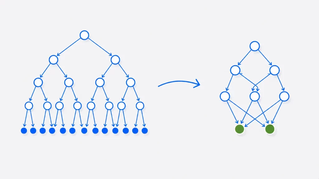
A binary decision tree becomes a Binary Decision Diagram by repeatedly applying two reduction rules until no more reductions are possible. These rules are what make BDDs compact:
Rule 1 — Merge identical terminals and isomorphic subgraphs. If two nodes have the same variable and their low edges point to the same subgraph and their high edges point to the same subgraph, they are duplicates — merge them into one shared node. This is why a BDD only ever needs a single “0” terminal and a single “1” terminal, no matter how many times they appear in the tree.
Rule 2 — Eliminate redundant tests. If a decision node’s low edge and high edge both point to the same node, then that variable doesn’t affect the outcome at this point — remove the node and redirect its incoming edges to that single child.
Applying these two rules repeatedly transforms the exponential decision tree into a much smaller directed acyclic graph that represents exactly the same function. The result, when combined with a fixed variable ordering, is the ROBDD.
Ordered and Reduced Ordered BDDs (OBDD and ROBDD)
BDDs come in several variants, distinguished mainly by ordering and reduction:
- Ordered BDD (OBDD). The variables appear in the same fixed order along every path from root to terminal. This ordering is what makes efficient manipulation possible.
- Reduced Ordered BDD (ROBDD). An OBDD with both reduction rules fully applied. This is the form most people mean when they say “BDD.” Its defining property is that it’s canonical: for a given function and variable order, the ROBDD is unique. That canonicity is what makes ROBDDs so valuable for equivalence checking.
- Zero-Suppressed BDD (ZDD). A variant optimized for representing sparse sets of combinations, widely used in combinatorial problems.
- Free BDD (FBDD). Drops the fixed-ordering requirement, gaining flexibility but losing canonicity and some efficiency.
One important caveat: the variable ordering dramatically affects a BDD’s size. For the same function, a good ordering can produce a tiny BDD while a bad ordering produces an exponentially large one. Finding the optimal ordering is itself an NP-hard problem, which is why real BDD libraries include heuristics for reordering variables.
BDD vs Binary Decision Tree vs Binary Search Tree
These three sound similar but are quite different structures — a common point of confusion.
| Feature | Binary Decision Diagram (BDD) | Binary Decision Tree | Binary Search Tree (BST) |
|---|---|---|---|
| Structure | Directed acyclic graph (shares nodes) | Tree (no sharing) | Tree |
| Represents | A Boolean function | A Boolean function | An ordered set of values |
| Node meaning | A variable test | A variable test | A stored key |
| Key benefit | Compact, canonical form | Simple, illustrative | Fast search/insert/delete |
| Size | Can be exponentially smaller than the tree | Exponential (2ⁿ leaves) | Proportional to items stored |
| Typical use | Verification, circuit design | Teaching, small functions | Lookups, sorted data |
The essential distinction: a BDD and a decision tree both represent Boolean logic, but the BDD shares identical subgraphs so it’s far more compact. A binary search tree is unrelated — it stores and searches ordered data, and has nothing to do with Boolean functions despite the similar name (which is exactly why “binary decision tree” searchers often end up confused).
The Apply Operation
The single most important BDD operation is Apply, which combines two BDDs with a Boolean operator (AND, OR, XOR, etc.) to produce a new BDD. It works recursively on the two graphs, following the shared variable ordering, and uses a cache of already-computed results so identical sub-problems are solved only once. This is what lets BDD packages combine complex functions efficiently — building up a large function from smaller ones without ever expanding to a truth table.
A BDD Example in C
The following C program builds a small decision-node structure for the Boolean function f = (a AND b) OR c and evaluates it for every possible input. It demonstrates the core idea — decision nodes, terminal nodes, and evaluation by traversal — though a production BDD package adds reduction, ordering, and node sharing through a hash table.
#include <stdio.h>
#include <stdlib.h>

typedef struct Node {
    int var;              // variable index: 0=a, 1=b, 2=c; -1 for a terminal
    int value;            // terminal value (0 or 1) when var == -1
    struct Node *low;     // edge taken when the variable is 0
    struct Node *high;    // edge taken when the variable is 1
} Node;

Node *terminal(int value) {
    Node *n = malloc(sizeof(Node));
    n->var = -1; n->value = value; n->low = n->high = NULL;
    return n;
}

Node *decision(int var, Node *low, Node *high) {
    Node *n = malloc(sizeof(Node));
    n->var = var; n->value = -1; n->low = low; n->high = high;
    return n;
}

// Evaluate by following low/high edges until a terminal is reached
int evaluate(Node *node, int a, int b, int c) {
    int vars[3] = {a, b, c};
    while (node->var != -1)
        node = vars[node->var] ? node->high : node->low;
    return node->value;
}

int main(void) {
    Node *T = terminal(1);          // single shared "1" terminal
    Node *F = terminal(0);          // single shared "0" terminal

    // Decision structure for f = (a AND b) OR c, order a, b, c
    Node *c_node = decision(2, F, T);
    Node *b_node = decision(1, c_node, T);
    Node *root   = decision(0, c_node, b_node);

    printf(" a b c | f = (a AND b) OR c\n");
    printf("-------+--------------------\n");
    for (int a = 0; a <= 1; a++)
        for (int b = 0; b <= 1; b++)
            for (int c = 0; c <= 1; c++)
                printf(" %d %d %d |        %d\n", a, b, c, evaluate(root, a, b, c));

    return 0;
}
Output:
 a b c | f = (a AND b) OR c
-------+--------------------
 0 0 0 |        0
 0 0 1 |        1
 0 1 0 |        0
 0 1 1 |        1
 1 0 0 |        0
 1 0 1 |        1
 1 1 0 |        1
 1 1 1 |        1
Notice how the single terminal nodes T and F are shared by multiple decision nodes rather than duplicated — that sharing is the essence of what makes a real BDD compact. A full BDD library extends this with a unique-node table (so identical subgraphs are automatically shared) and the two reduction rules.
Applications of BDDs
BDDs are used across computer science and engineering wherever Boolean functions need to be represented and manipulated efficiently:
- Formal verification and model checking. BDDs are a foundation of symbolic model checking, used to verify that hardware and software systems behave correctly by representing enormous state spaces compactly.
- Digital circuit design. In electronic design automation (EDA), BDDs are used for logic synthesis, optimization, and equivalence checking — confirming that an optimized circuit computes the same function as the original.
- Software analysis. BDDs power some static analysis tools that detect bugs and vulnerabilities by reasoning about program logic.
- Artificial intelligence. BDDs are used in knowledge representation, symbolic reasoning, and AI planning, where large sets of states or constraints must be handled efficiently.
- Combinatorial optimization. ZDDs, the sparse-set variant, are used to represent and count combinations in problems like network reliability and constraint solving.
Tools and Libraries for BDDs
You rarely implement BDDs from scratch for real work — mature, highly optimized libraries handle reduction, ordering, and node sharing for you:
- CUDD (Colorado University Decision Diagram package). The most widely used C/C++ library for BDDs, ADDs, and ZDDs, used heavily in academia and EDA tools.
- BuDDy. A well-known, lightweight BDD library for C and C++, popular for teaching and research.
- Sylvan. A modern, multi-core parallel BDD library for high-performance applications.
- PyEDA. A Python library for electronic design automation that includes BDD support, convenient for experimentation.
- JavaBDD. A Java library for BDD manipulation, often used in program analysis tools.
Frequently Asked Questions
Conclusion
Binary Decision Diagrams are one of the most elegant data structures in computer science: by sharing identical subgraphs and eliminating redundant tests, they compress Boolean functions that would otherwise be impossibly large, while keeping the ability to operate directly on the compressed form. The reduced ordered form (ROBDD) adds canonicity, turning the hard problem of checking whether two Boolean functions are equal into a simple graph comparison — which is why BDDs became foundational to formal verification and circuit design.
For deeper study, explore the classic BDD libraries like CUDD, and see how BDDs sit alongside Trie data structure and other data structures in our guides to data structures and algorithms.